Using Machine Learning to Parse Web Pages Into Semantic Sections
Around two months ago, I joined forces with the rest of the teleportHQ team in our mission to reduce friction and eliminate dead ends in the GUI building process, spawning a machine learning (ML) track. Most of the team focuses on building tools for designers and developers to bridge the gap between these two roles. They do this by facilitating a common medium and ideation environment. The first tool we developed, aimed at designers, is a Sketch plugin that exports code. You can read about it over here, in an article by our CTO, Criss.
Yet we want to take it one step further. In the not-so-distant future, we aim to go beyond designers and developers. And we want to target the non-technical person. We want to provide the right toolset so that someone with business skills, but no design or coding knowledge, will be able to create a beautiful website or app with relative ease.
This overarching ideal was clear from the beginning. But we had no clearly defined problem to address through machine learning (ML). And we had absolutely zero data to train ML solutions on…. Well, no data except the whole raw, loosely structured, and unprocessed world wide web; one of the biggest data sets in the entire world. So, what would a data scientist do with all this spaghetti bowl of html, JavaScript and CSS? Panic.
.
Finding Structure in Chaos
We took a step back and started brainstorming for a bit… What if we’d mine the web to discover certain rules, by calculating ratios and finding formulas and complex relationships between properties of various elements? How about using these rules to forward suggestions to the user that’s building his website? For instance, we’d build the distribution of ratios between the font size of a menu button and its margin and padding. Or the spacing between menu items in relation to the size of the menu and the size of each individual item. We’d then take these trends and suggest them to be applied on whatever our non-designer user is building.
One issue though… What’s a menu?
Well, it’s obvious, you might say, it’s the list of items that serve navigation purposes. And while you would be very right, something that is obvious and trivial for us, humans, is anything but for a computer algorithm. If we visit a web page we can immediately visually distinguish all the page elements, and understand the content. If we were to use a web crawler to compute our fancy formulas, it wouldn’t know the concept of a menu. So let’s start from here. It seems like solving this problem would enable us to make some context-aware queries on the world wide web. Let’s teach an algorithm to identify certain key sections within a web page. It would be quite useful to find the meaning of various elements; their semantic value within the HTML document.
This task would indeed be trivial for a crawler too if we lived in a perfect world where everybody would use the semantic elements introduced in HTML5. These tags were introduced to address this exact problem: to ease the automated processing of websites. Unfortunately, these elements are less widely spread than needed.
Here are the new semantic tags introduced in HTML5:
.
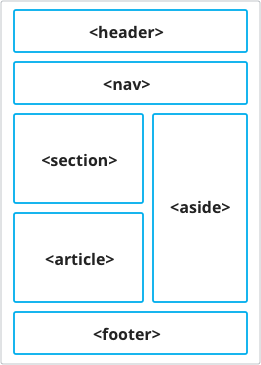
<article>, <aside>, <details>, <figcaption>, <figure>, <footer>, <header>, <main>, <mark>, <nav>, <section>, <summary>, <time>
Starting from these tags we’ve defined our own main semantic sections. It’s an annotation that aims to be a simplification of the HTML5’s semantic elements, while yielding a rough blockout of the web page. The sections we ended up defining are:
- nav
- header
- content
- footer
- control
- form
We’ve kept the nav, header, and footer from the HTML5 notation. And we aggregated a bunch of the other tags under the content section. We’ve also included the form semantic tag and defined a new section control. Control is meant to define any menu bar or toolbar which contains a set of inputs used to sort or filter data.
The process of identifying the semantic meaning of an HTML element can be viewed as a classification problem that can be solved through supervised learning. If you know how supervised machine learning works (even if superficially), then you know that in order to train a model you require large amounts of annotated data in order for your model to learn the labels that you are trying to predict for each element.
But nobody wants to go through thousands of websites and manually annotate each and every section… So we’ve built a Chrome extension to partially automate the process by pre-parsing the website based on a collection of heuristics.
Defining heuristics
“A heuristic, is any approach to problem solving, learning, or discovery that employs a practical method, not guaranteed to be optimal, perfect, logical, or rational, but instead sufficient for reaching an immediate goal.”
— Wikipedia
It was clear that we didn’t want to make all of this labeling work manually. We’ve started to dissect what makes us think that a certain element obviously serves a certain function. What makes a nav bar a nav bar? Well… it’s usually a list, it contains anchor tags. It’s either a long horizontal element in the top part of the page or a vertical one on the left. We might find certain keywords within its inner HTML and so on and so forth…
Based on these rules we can then define a scoring function for how nav-like an element is. Such a function could look something like:
navScore = 0.5 * containsTags(<UL>, <OL>, <LI>)
+ 0.3 * containsTags(<A>)
+ 0.2 * containsKeywords(‘nav’, ‘navigation’, ‘menu’)
.
Of course, this is an oversimplified example of what we ended up using. We’ve implemented these inner functions (containsTags, containsKeyword, etc) in JavaScript and called them evaluators. The number multiplied with these functions are weights that we empirically adjusted to give more importance to certain properties. Then, we repeated the process for every section we defined. And we wrapped everything nicely in a Chrome extension that gives the human annotator an initial parsing of the page and allows further finer control over the section configuration.
.

.
Gathering data
Now that we have the parsing or the annotation of the website, how do we save it? There are three main ways to do it.
- Save a rendered image with bounding rectangles for each website.
- Save the entire HTML with some extra info related to where the section are.
- Do a bit more work and compute some meaningful features and save tabular data.
The first solution works if we deal with visual information. But in the context of a crawler, we’d have to render the page, get the bounding boxes, and then map the result over the HTML elements, which is quite a bit of an overhead. Both of the first two approaches also raise some privacy concerns for the annotators using the extension. For instance, if they’d parse their Facebook feed, we wouldn’t really want to store pictures of their friends and other sensible information.
The best solution in our case is extracting the exact features (or properties) that we’d need to train a machine learning model on. Remember the example scoring function from earlier? We could make an algorithm to learn those weights, rather than having us manually tweaking them. And it can learn these weights automatically for all the section.
All we’d need to do is compute all possible properties for each element. For instance, given that we’re checking containsTags(<UL>, <OL>, <LI>) for nav and containsTags(<IMG>, <SVG>), we will compute for all elements 5 features: containsTags(<UL>), containsTags(<OL>), containsTags(<LI>), containsTags(<IMG>), containsTags(<SVG>) and then feed all of these properties to a machine learning model. Other properties that we considered to be quite relevant were coordinates returned by getBoundingRect, normalized to window height and width.
We ended up computing 195 features for every element and storing them in a csv file in the following format:
<index, url, features, label>
.
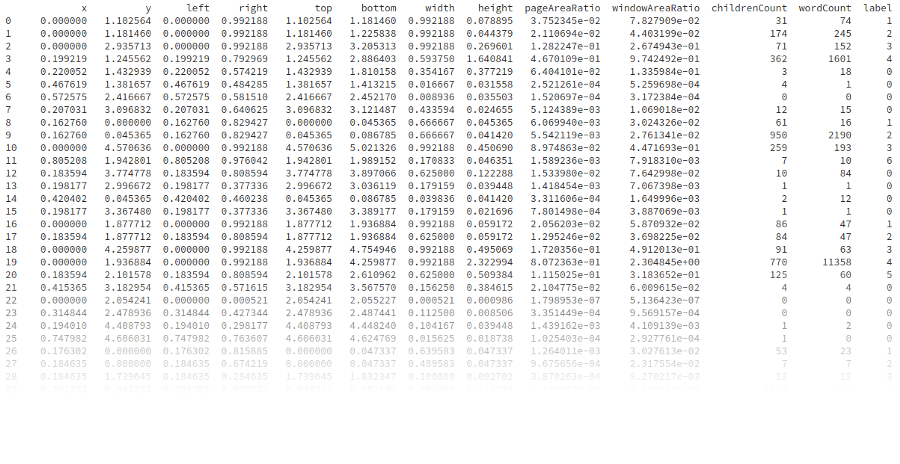
A few of the computed features. Now we can start talking ML!
In order to reduce the number of false positives, we had to add a new category besides the aforementioned sections — a “no section” label. We added to the data set one negative example for every section parsed. The negative examples are randomly chosen from the HTML elements in the page that are not selected as being a section.
We also wanted to use a similar model to identify a user’s intent, or rather what he was building in sketch, or in another tool at a given time. For instance, we would like to know if a user is currently putting together a menu, to forward relevant suggestions to him. Unfortunately, most of our 195 features would not be relevant in the context of a design tool. So we’ve selected a subset of these features that are available within such tools (positioning, bounding box, size, area, children count, etc) and trained our model on this smaller data set as well.
Training a section classifier
If you’re new, a complete stranger, to machine learning, I encourage you to read this post by Sam Drozdov, An intro to Machine Learning for designers. You don’t even have to be a designer to read that post. It is quite general, comprehensive, and a very good overview of the field. For a more business-oriented approach, there is this video by Andrew NG which is a very good first contact with ML.
This part of the article will be more technical and harder to digest. So brace yourselves!
.
.
We ended up training three algorithms on the data we’ve collected: a support vector machine, a neural network, and an XGBoost classifier in order to find the best fit for addressing our problem. I will take the next few paragraphs to briefly talk about the algorithms, the hyperparameters we’ve used, and our results.
Support vector machine (SVM)
Support vector machines are generally a pretty difficult concept to grasp for non-math-geeks. In essence, SVMs are mathematical models that divide data points into classes by finding a hyperplane that separates them in the dimensional space of their features. A hyperplane is a subspace of an n-dimensional space that has n-1 dimension. For instance, a hyperplane for a 2D space would be a 1D line and a hyperplane for a 3D space would be a 2D plane.
In the example in the figure above, the points are the data entries. Their colors are their labels (label = class). X₁ and X₂ are the features of these entries (of which we have 195) and also represent the spatial dimensions of the model. H₁, H₂, H₃ are all hyperplanes in this 2D space. SVMs are trying to learn the hyperplane that separates the data with the largest margin (in this example H₃). The samples closest to this hyperplane boundary are called support vectors, hence the name.

We’ve trained an SVM on our data, using a linear kernel and a one vs. many multiclass classification strategy (innately SVMs are binary classifiers, they find hyperplanes that can separate two classes). We’ve chosen a linear kernel because it was proven to work well in high-dimensional spaces using no dimensionality reduction techniques (Kernel Selection and Dimensionality Reduction in SVM Classification of Autism Spectrum Disorders). If you’re math savvy, yet you find these issues hard to understand although you would like to, please give this lecture on SVMs from MIT a try. The rest of the SVM parameters are the default ones from sklearn.
Neural Network (NN)
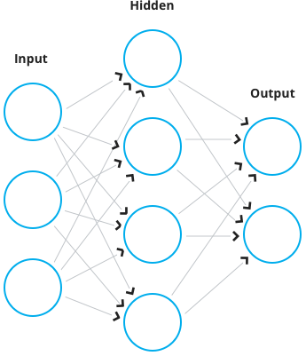
Artificial Neural Networks (ANN) are loosely modeled after the human brain. They consist of interconnected neurons that ‘process’ information. This processing usually means the aggregation of some inputs, feeding the aggregated value into a function and then broadcasting it to other neurons. Most ANNs have a minimum of three layers. The input layer, in which the data is being plugged, one or more hidden layers are used for computations, and an output layer from where we can read the result.
.
.
If we want to solve a classification problem using ANNs, the number of neurons on the output layer will equal the number of classes we’re having, each neuron corresponding to one class. The output of a given neuron is the probability of the processed data entry to be of that specific class if using an output layer such as softmax. If you’re a complete stranger to how neural networks work, 3Blue1Brown has a couple of videos that explain the concept: video 1, video 2.
For our experiments, we used 5 hidden, fully connected (fc) layers in the following configuration (the number in front of the layer type is the number of neurons on the layer):
.
195 input → 2x 512 fc → 2x 256 fc → 128 fc → 7 softmax
.
We used an early stopping training strategy and each fully connected layer was followed by a dropout layer in order to prevent overfitting (given that we did not have, at the moment of training, too many entries in our data set). We used the leaky rectified linear unit (ReLU) function as the activation function for each layer. The network was built using Keras with a Tensorflow back-end.
Extreme Gradient Boosting (XGBoost)
XGBoost, is quite an interesting take on supervised learning. It’s an ensemble method, which means it consists of a bunch of smaller, weaker (less performant) classifiers that together draw the “right conclusion”. XGBoost is a decision tree ensemble model. Luckily, at an intuitive level, decision trees are quite easier to understand as they maps quite well on our decision-making process. For instance, if we want to estimate how likely it is for an HTML element to be a navigation bar, we’d end up with a decision tree looking something like this:
[/fusion_text]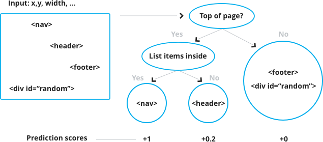
But this is a single decision tree. Using a single tree is not strong enough to be used in practice. So in order to get a better prediction, we sum the output of multiple trees together.
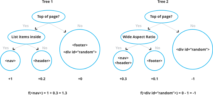
The method of using such randomly constructed tree classifier put together is called a Random Forest. XGBoost builds onto this concept by finding a more information-theory driven method for building the trees in the ensemble. I won’t go into further details, but if you want to read more about XGBoost, you can do so here.
.
Results and comparison
In order to illustrate our results, we will use the concept of confusion matrix, also known as error matrix. The rows of the matrix represent instances in their ground truth class, while the columns depict the predicted labels for those classes. For instance, if we take a sneak peak at the next figure, the first matrix, we can read from it that the SVM misclassified 34% of the headers as being non-sections and 11% as being navigation bars.
The matrices were computed after running 10-fold validation on the entire data set. This means that we retrained from scratch each model 10 times on 90% of the data while testing on the rest of 10% that did not go into training at that step. Then we averaged all results over these runs to compute the final numbers.
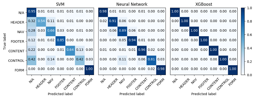
As we can see in this figure, SVM had some bias issues towards the “non-section” class, as it was the class most prevalent (5:1) in the data set. As previously stated, this is the result using class weights in order to compensate for this ratio, yet apparently it was not enough. The neural network did fairly good, struggling a bit on the “control” class, which is not surprising, given that this class has quite a loose definition. Astonishingly, XGBoost scored a perfect 1, which might be due to the fact that most of the features are sparse and discrete, making splitting (defining ‘if’ rules in the decision trees) efficient in classifying the data.
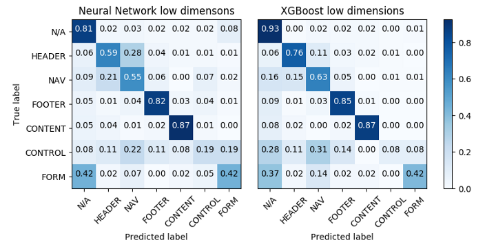
Confusion matrices for the low-dimensional data set. The SVM classifier failed to learn anything meaningful.
The results on the small feature set are quite poor for all models, XGBoost coming slightly ahead. SVM did not manage to fit the data, while the neural network and XGBoost failed to learn the “control” and “form” classes. This is not very surprising as those classes are not really defined by their positional features, but rather by their contents.
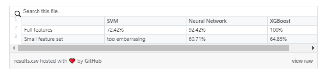
Mean accuracy for every model.
We’ve put together a small repository containing the data we used, in a csv format, and a jupyter notebook with the code needed to train the classifiers yourself. Feel free to tweak the hyperparameter used and try and get better scores!
Conclusion and future work
In large we’ve accomplished our initial goal of designing the “brain” of a semantics-aware crawler. Of course, there’s still a lot of work that could be done: using grid search to select optimum hyperparameters for the models, designing a better neural network, gathering more data, and putting together an ensemble of different kinds of models to compute a more accurate final result. And the most important thing would be to test the trained models on unseen data and observe how it performs. I have the feeling that the XGBoost model is not as perfect as it lets us believe. 🙂
Not sure when we’ll get to do all of these things, as this direction of experimentation is for now on halt. We’ve started to focus on a way more interesting application of ML for teleportHQ. We’ll have an important announcement to make on this quite soon.
So make sure to stay tuned! Follow us on Twitter and Medium to be the first one to find out!
Signing out,
– Raul Incze